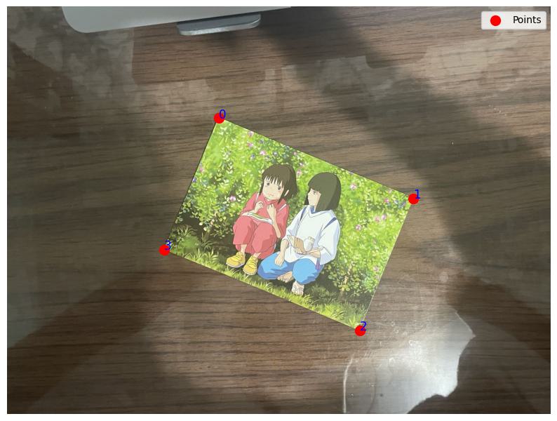

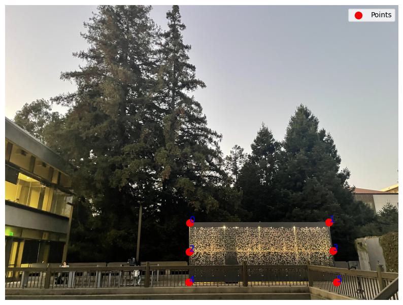
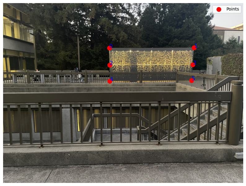
In this step, I implemented a function to compute the homography matrix. It takes the corresponding points from two images as parameters and calculates the homography matrix. According to the definition, the relationship can be expressed as:
$$ A \cdot h = b $$
Here, \( A \) is a matrix that is constructed using the coordinates of the points from the source image. For each pair of corresponding points \( p = (x, y) \) in the source image and \( p' = (x', y') \) in the destination image, we can define the matrix \( A \) for a single point as:
$$ A = \begin{bmatrix} x & y & 1 & 0 & 0 & 0 & -x' \cdot x & -x' \cdot y \\ 0 & 0 & 0 & x & y & 1 & -y' \cdot x & -y' \cdot y \end{bmatrix} $$
The vector \( b \) represents the destination points, and is defined as:
$$ b = \begin{bmatrix} x' \\ y' \end{bmatrix} $$
For multiple points, I append additional rows to both \( A \) and \( b \). After solving the system of equations \( A \cdot h = b \), I recover the homography \( h \) and reshape it into a \( 3 \times 3 \) matrix \( H \).
I utilized the warp function that I previously implemented in project 3. In this task, I modified the function to work with homographies for more flexible transformations. For image rectification, I retained the polygon mask to focus the transformation on specific regions.
For mosaic image stitching, I developed a new warp function without a polygon mask to stitch images from different angles. I calculated the grid coordinates of the target image, applied the homography, and performed inverse mapping. I also applied a validity check and bilinear interpolation to ensure correct pixel placement.
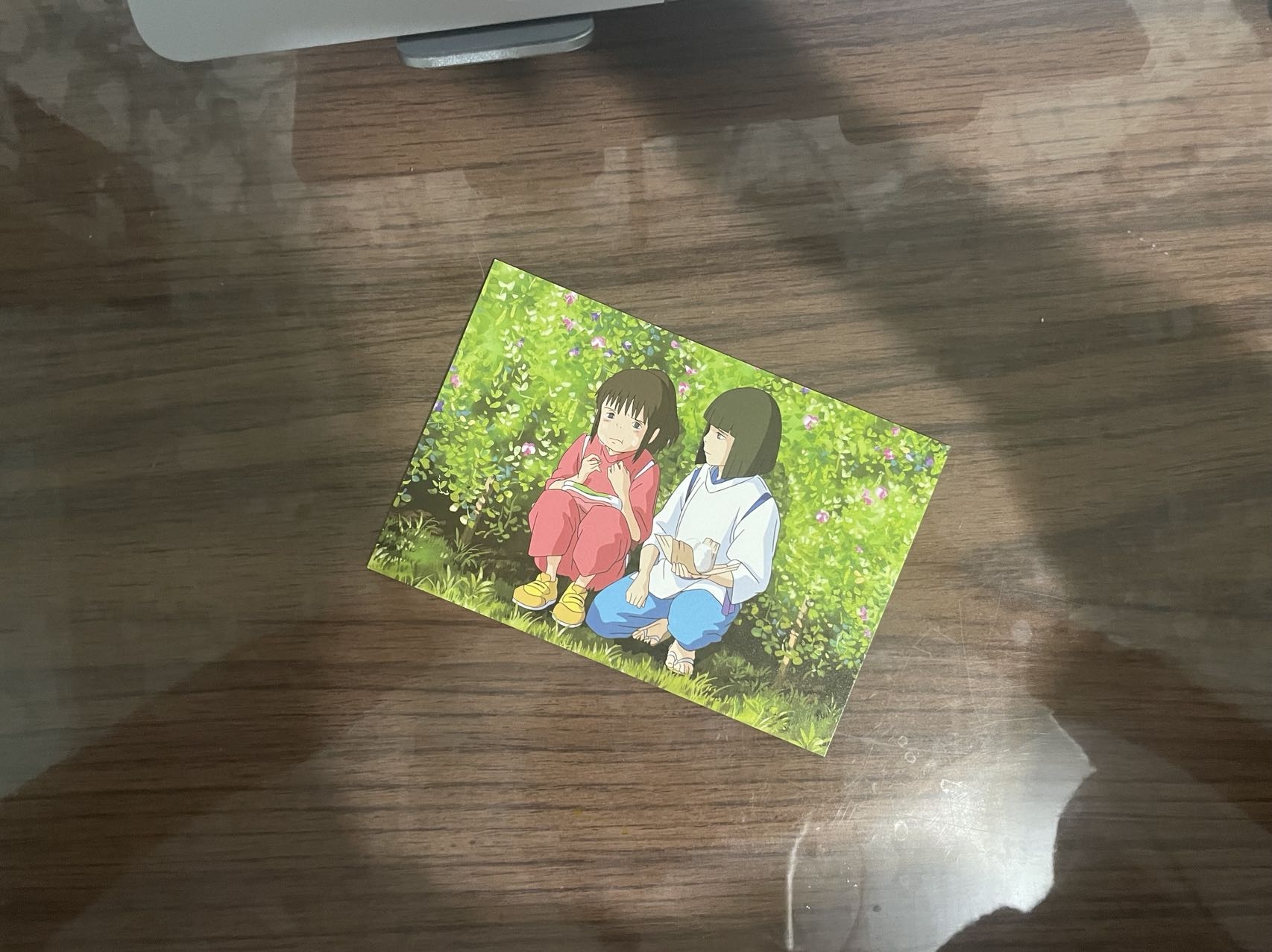
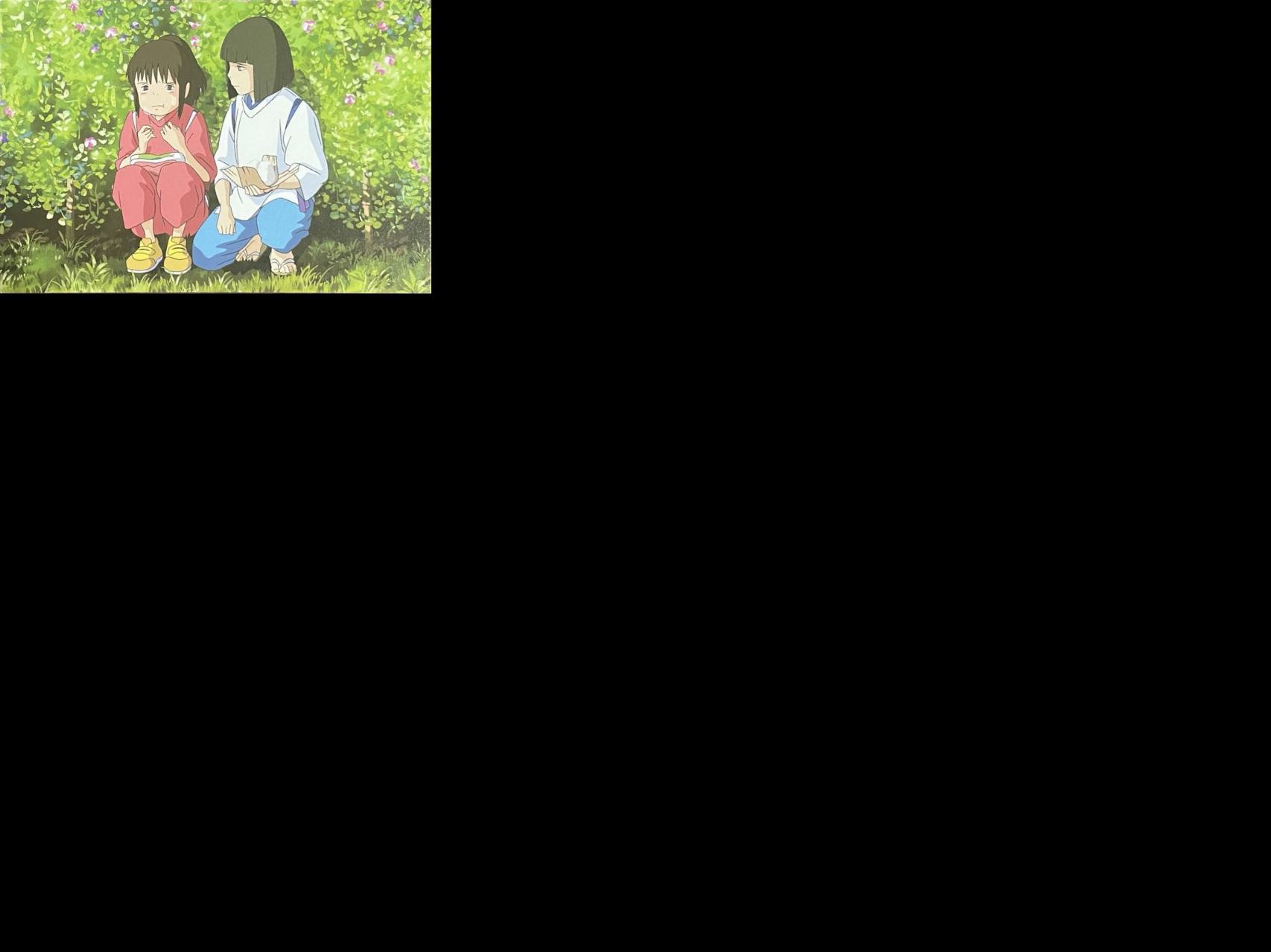
I marked the corners of the poster in the image, computed the homography to transform the poster into a rectangular form, and applied interpolation to assign pixel values smoothly.
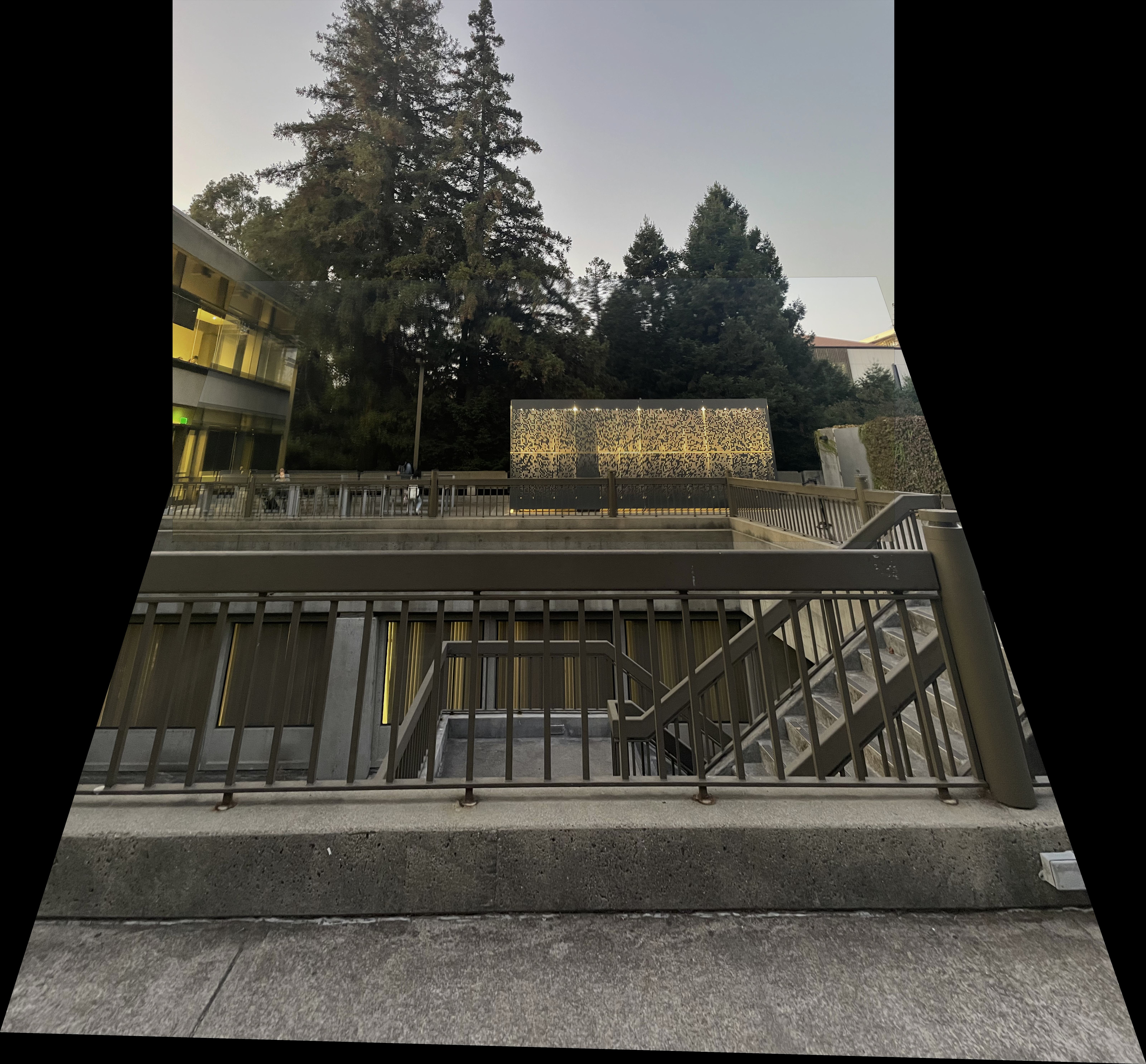
First, I used the ComputeH function to calculate the homography matrix between two images. Then, I computed the boundary of the mosaic canvas to ensure it was large enough to fit both images. A translation matrix was applied to adjust the images' positions. Finally, Gaussian-blurred masks ensured smooth blending between the stitched images.
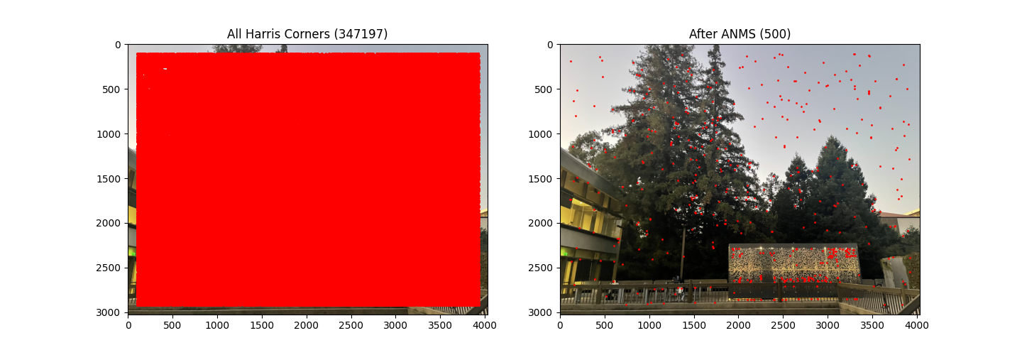
After running the get_harris_corners function, we obtain an image densely packed with detected feature points.
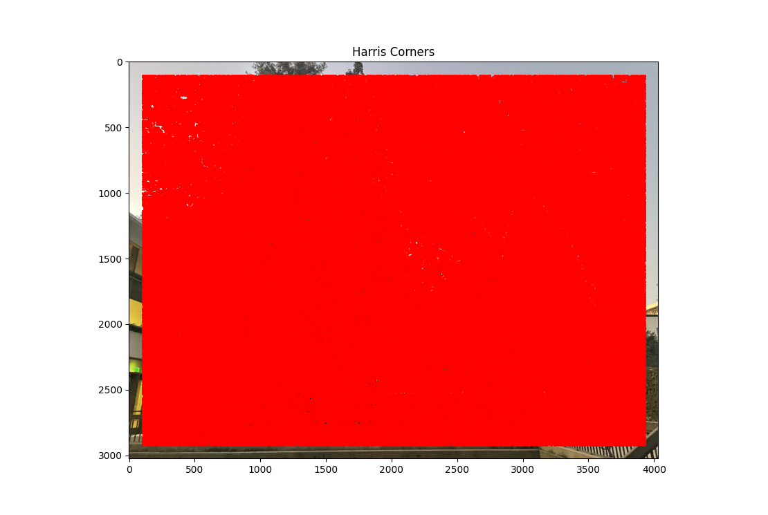
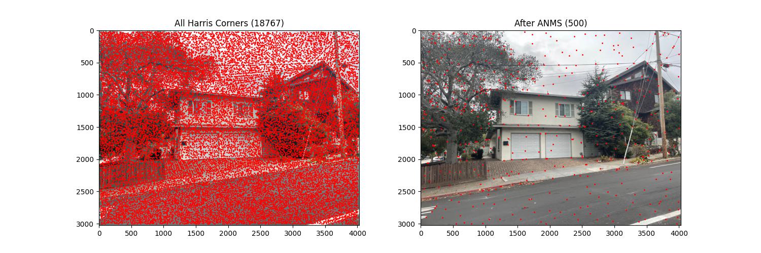
After running get_harris_corners, we get too many feature points in the image. To address this, I tried two methods:
min_distance parameter to maintain a minimum distance between feature points.threshold_rel parameter in the peak_local_max function to select stronger feature points and filter out the weaker ones.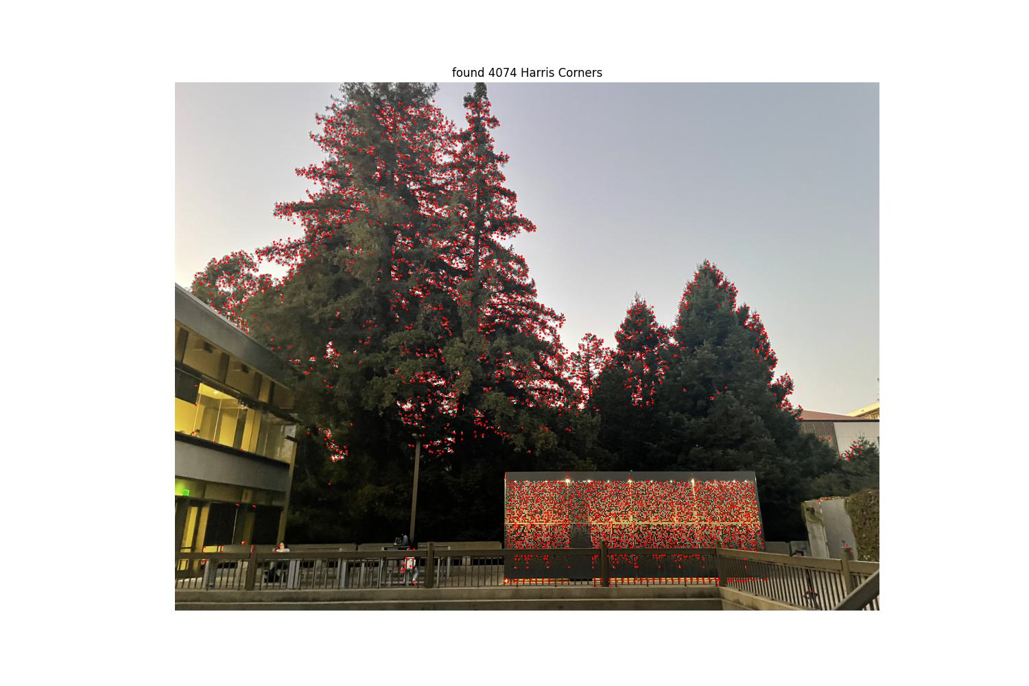
After my improvement, the feature points were still not evenly distributed. This issue was resolved by implementing the ANMS algorithm as described in the paper.
The core idea of this algorithm is to compute the minimum distance between each feature point and any "stronger" feature point, then keep the point with the maximum minimum distance. This ensures retained points are not only strong but also evenly distributed.
For each feature point selected through ANMS, we need to extract its feature descriptor. Based on the paper’s recommendations, I used the following method:
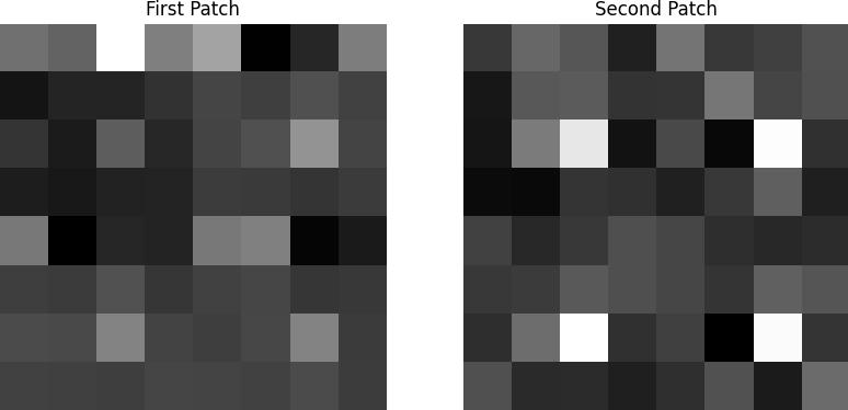
For feature matching, I applied Lowe's ratio test: the reliability of a match is determined by the distance ratio between the nearest and second-nearest neighbors.
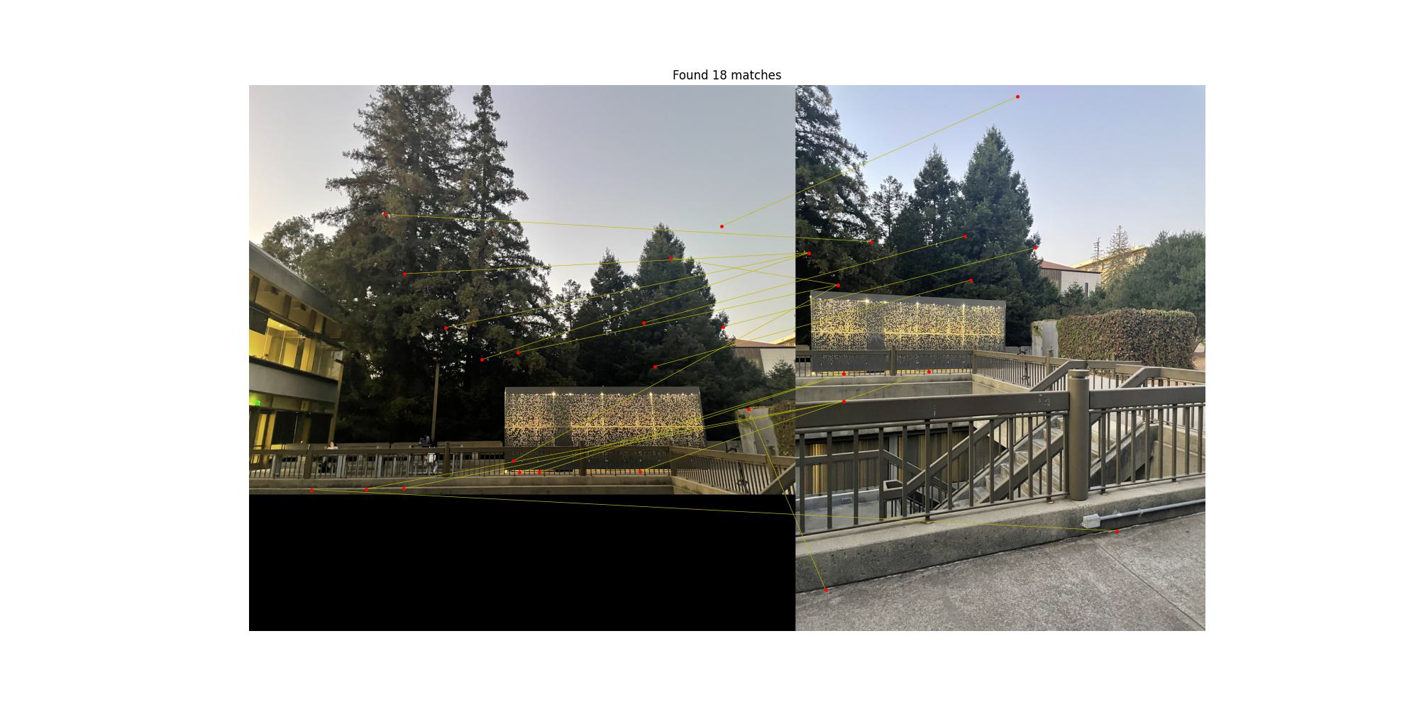
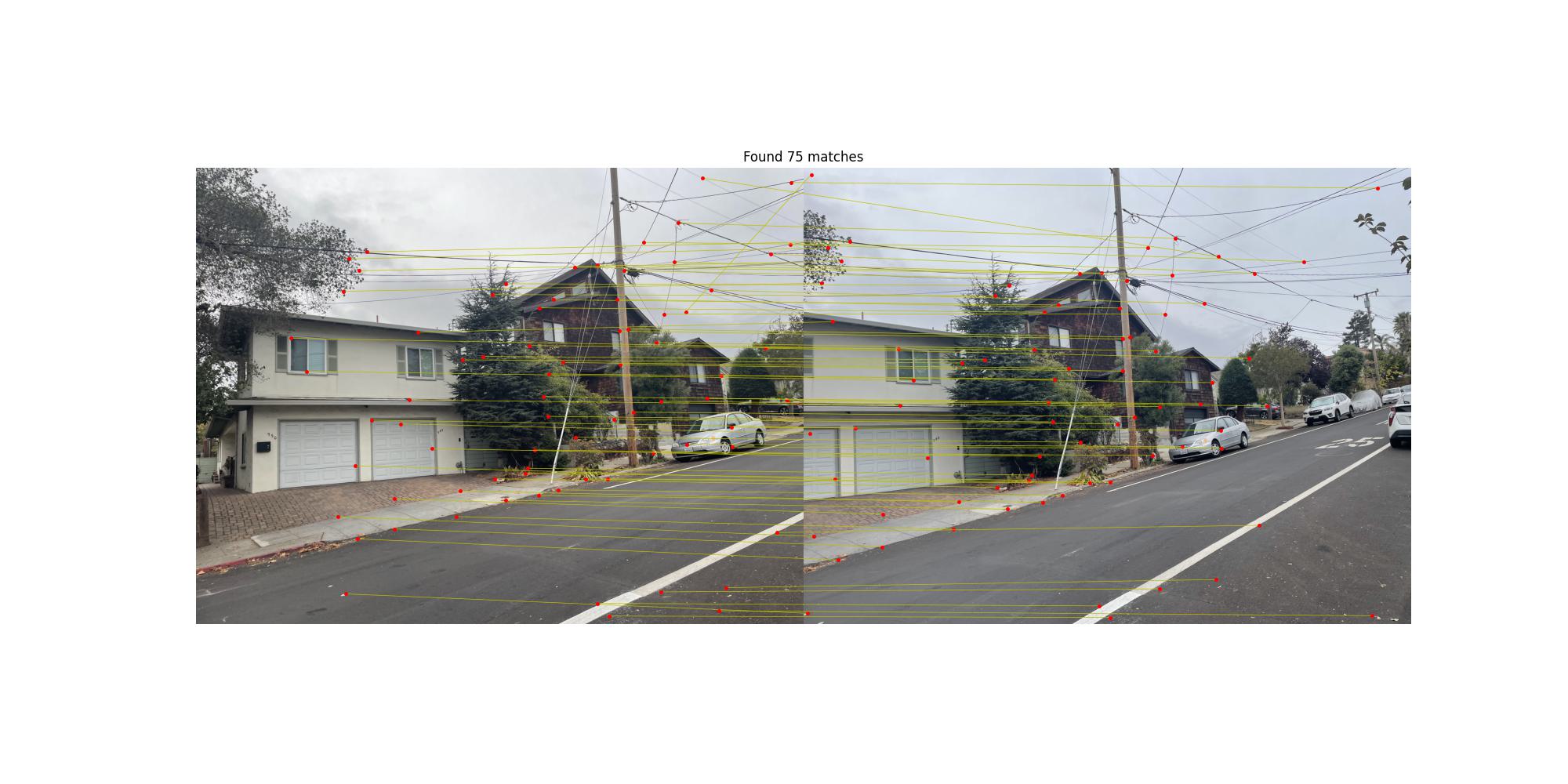
There are many obvious wrong matches, probably because of repeated patterns in the image.
To remove incorrect matches, I implemented the RANSAC algorithm. This algorithm iteratively samples random points to find the optimal homography matrix and identifies inliers that conform to this transformation.
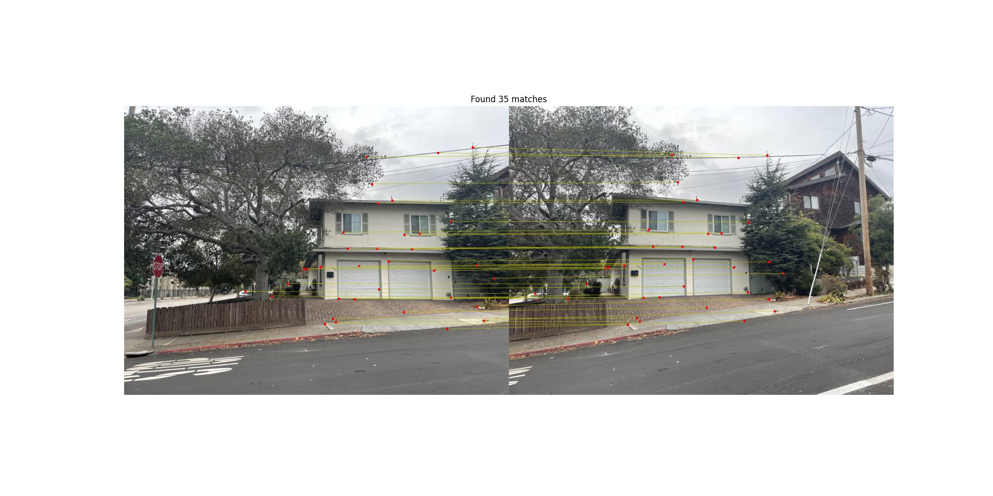
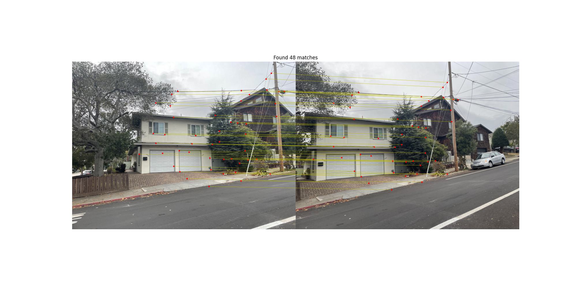
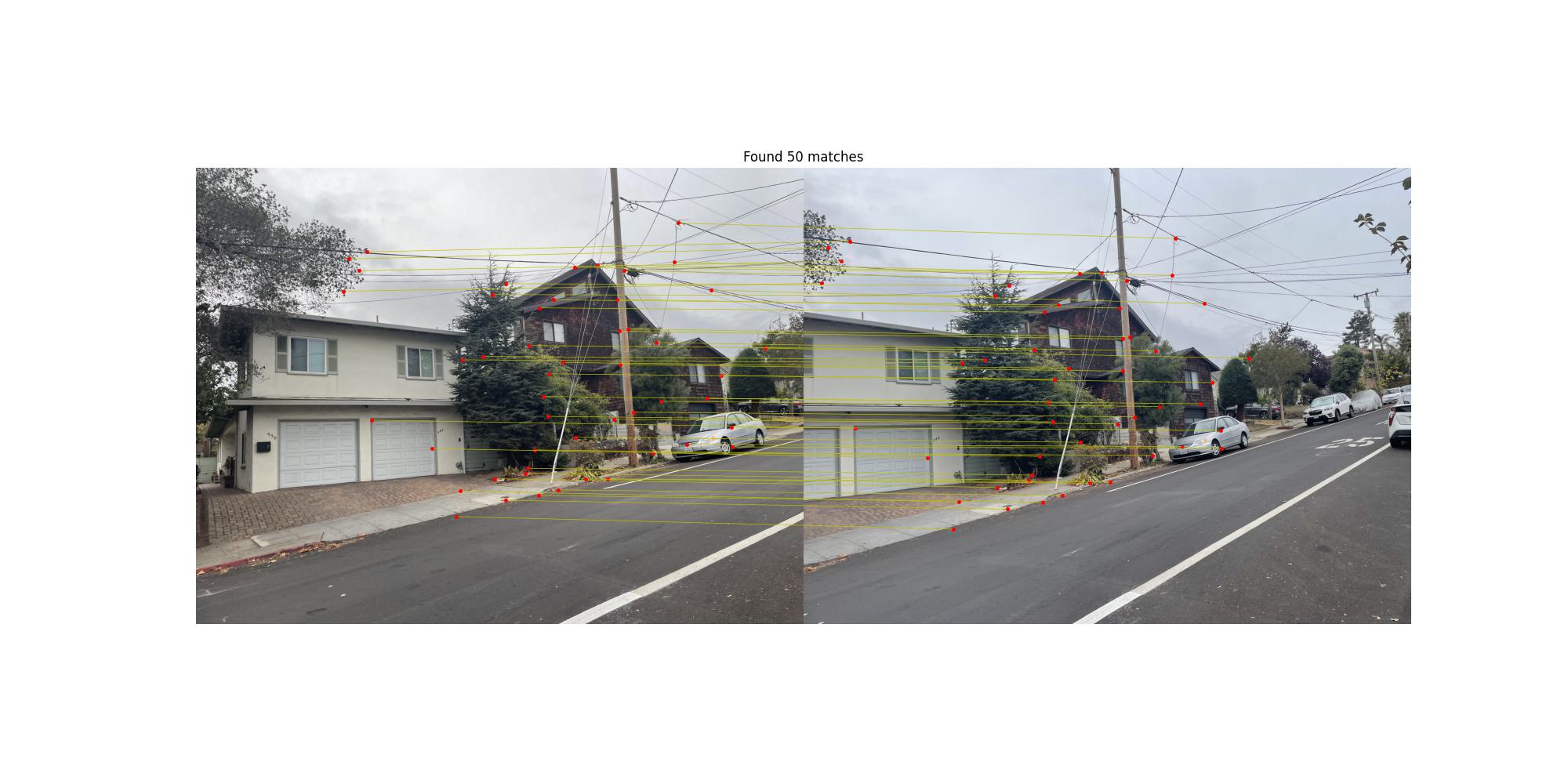
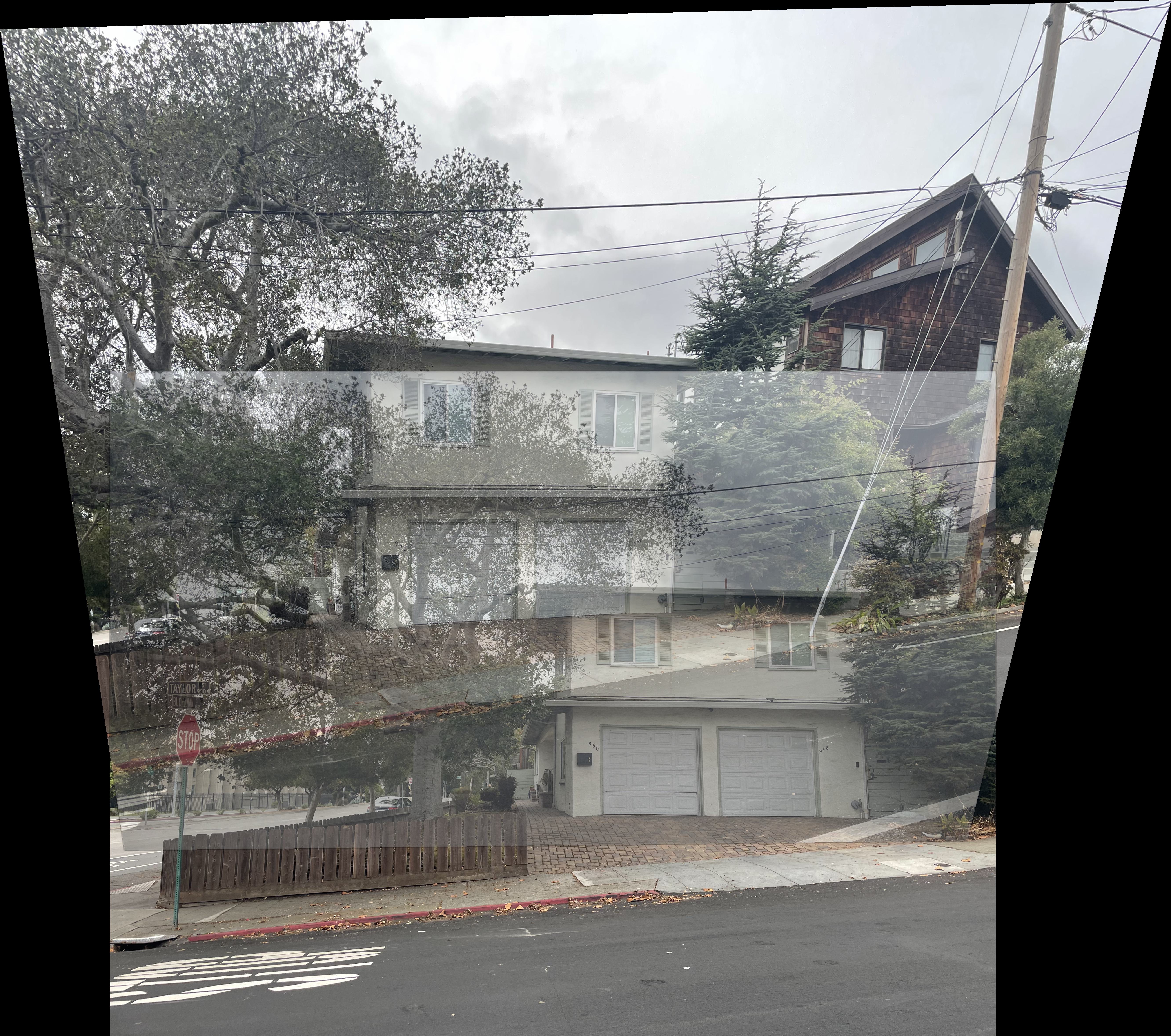
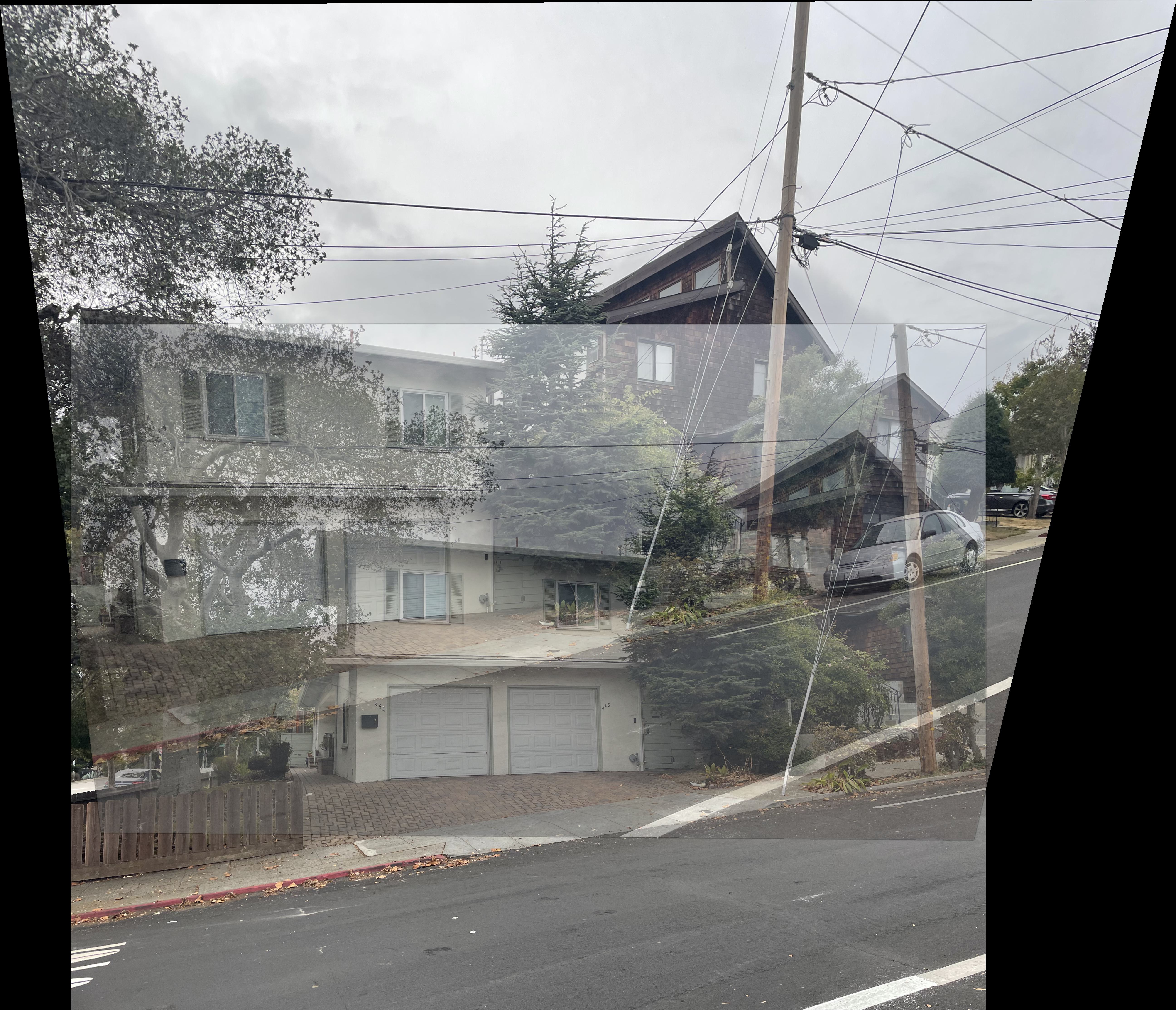
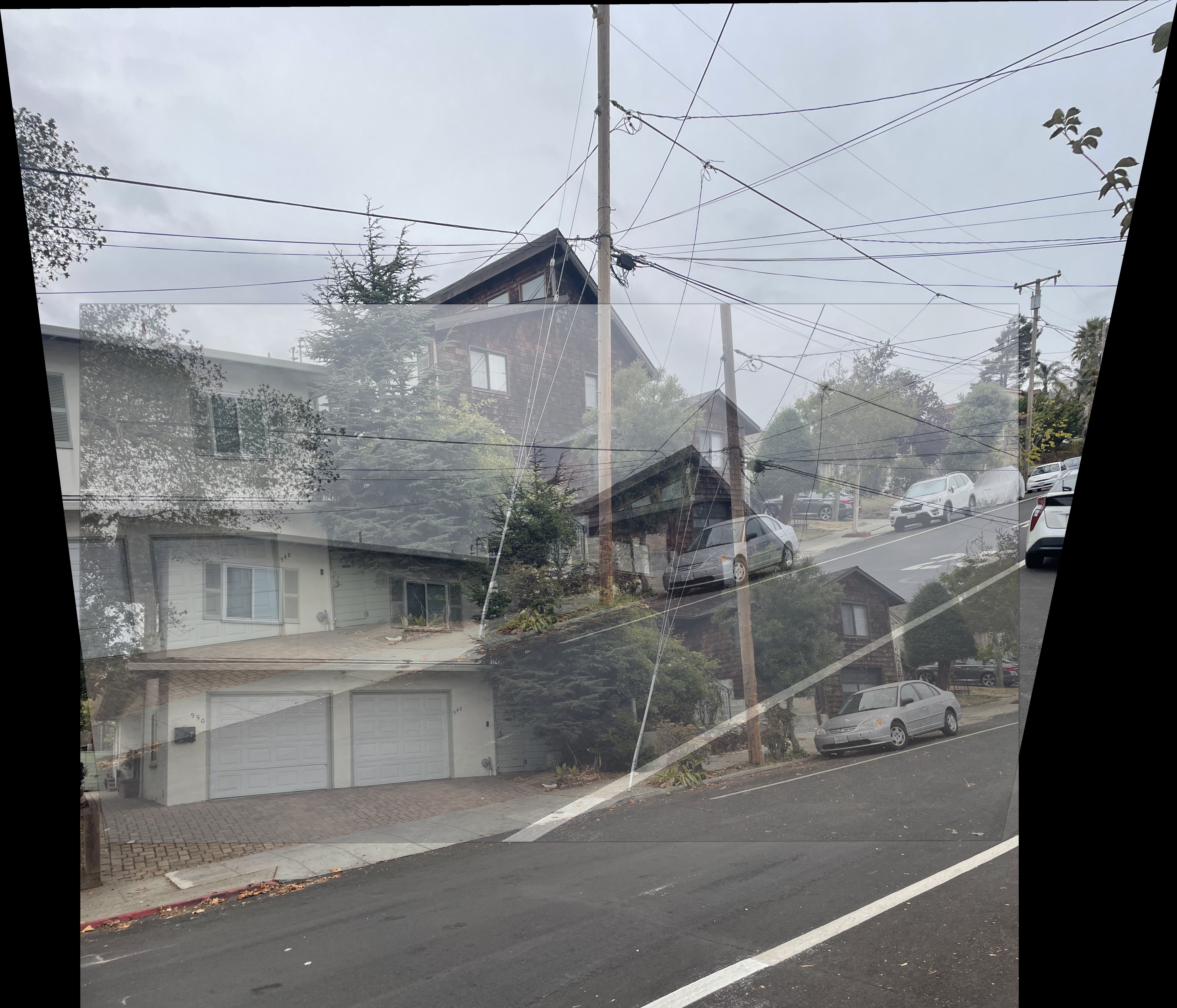
There are few issues we can see from the images.
The first issue is the misalignment in image stitching, where image elements are not precisely aligned. This is likely due to insufficient precision in feature point matching. Specifically, my ransac_homography function implementation may not be robust enough to effectively filter out high-quality matching point pairs.
The second issue is the lack of natural blending in image fusion, resulting in abrupt transitions at the stitching boundaries. This is primarily because I only used simple Gaussian blur for blending, rather than adopting a more advanced multi-resolution pyramid fusion method, which prevents me from effectively handling image details at different frequency levels.
The most exciting thing I learned from this project was the ANMS algorithm discussed in the paper. Initially, my approach was intuitive: select points with higher intensity. I tried various methods to improve the get_harris_corners function, such as increasing the min_distance parameter or setting a threshold for stronger feature points. However, these methods didn’t produce satisfactory results.
Implementing ANMS provided a better solution. Its core idea is not merely finding the 'strongest' points but ensuring a uniform distribution across the image. This reminded me of other fields, such as maze generation algorithms, where a similar approach divides large terrains into smaller sections before processing. Although I had encountered this 'spatial balancing' concept in other contexts, seeing its new application here was a pleasant surprise. It proves once again that good algorithmic ideas are often universal and can be applied flexibly.